Airline Connections Demo/Tutorial

This tutorial provides detailed information and instructions for the Airline Connections demo, which is built in to Hazelcast Cloud Trial.

Context

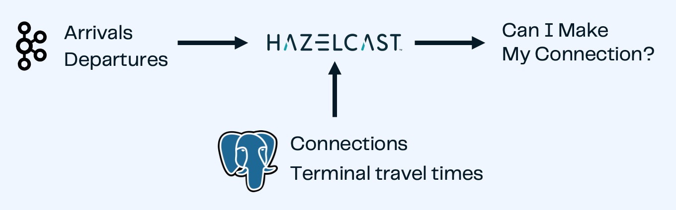
This demo/tutorial creates an application that uses streaming data about flight arrival and departure times, and correlates it with stored data about connecting flights, airport gates, and gate-to-gate travel times to determine whether there’s enough time to make a particular flight connection.

Connections Diagram

Specifically, you will learn how to

Connect to external data sources and sinks
Use SQL to search and display streaming data
Use SQL to import data from an external database
Configure late event handling for streaming data
Join streaming and stored data to generate continually updated results
Submit a job to Cloud using the Command Line Client

When you launch the demo in Cloud, you might see a step-by-step guide appear in conjunction with the demo. This tutorial is designed to supplement that guide, providing additional context and detail as well as links to reference materials. You can launch the step-by-step guide at any time by selecting the Walk me through this Demo link above the SQL browser.

Before you Begin

Before starting this tutorial, make sure that you meet the following prerequisites:

You have a running cluster in Cloud
You’ve downloaded and connected the Command Line Client to your cluster
For the client, you will need
- Java 17 or later
- Maven 3.9.0 or later
(Optional) Java IDE to view client code

Step 1. Review What’s Already Set Up

Begin by selecting the Airline Connections demo from the Cloud dashboard. This launches a pre-set configuration and opens the SQL browser window.

The pre-set configuration includes the following elements:

Connections to a Kafka server and a Postgres database
Mappings for streaming data
Mappings for IMaps to hold contextual data
Data imported from Postgres to local IMaps

Manual Set Up

To illustrate how the pre-set configuration would be done in the console, we provide the details below.

The best way to build connections to external sources is to use the Connection Wizard, which guides you through the steps needed to connect an external data source. You can then set up the mapping to make the external data available to the Hazelcast SQL engine

Walkthrough of Connection Wizard

The SQL code for each element is below.

Connect to the Kafka server:

CREATE OR REPLACE DATA CONNECTION TrainingKafkaConnection
     TYPE Kafka
     NOT SHARED
     OPTIONS
          ('bootstrap.servers'='35.88.250.10:9092',
          'security.protocol'='SASL_PLAINTEXT',
          'client.dns.lookup'='use_all_dns_ips',
          'sasl.mechanism'='SCRAM-SHA-512',
          'sasl.jaas.config'='org.apache.kafka.common.security.scram.ScramLoginModule required
          username="training_ro" password="h@zelcast!";',
          'session.timeout.ms'='45000'
          );

Mappings for streaming data:

CREATE OR REPLACE MAPPING "arrivals"
--topic name from Kafka
EXTERNAL NAME "demo.flights.arrivals" (
    --fields in topic
  event_time timestamp with time zone,
  "day" date,
  flight varchar,
  airport varchar,
  arrival_gate varchar,
  arrival_time timestamp
)
DATA CONNECTION "TrainingKafkaConnection"
OPTIONS (
    'keyFormat' = 'varchar',
    'valueFormat' = 'json-flat'
);

CREATE OR REPLACE MAPPING "departures"
--topic name in Kafka
EXTERNAL NAME "demo.flights.departures" (
    --fields in topic
  event_time timestamp with time zone,
  "day" date,
  flight varchar,
  airport varchar,
  departure_gate varchar,
  departure_time timestamp
)
DATA CONNECTION "TrainingKafkaConnection"
OPTIONS (
    'keyFormat' = 'varchar',
    'valueFormat' = 'json-flat'
);

Postgres database connection:

CREATE OR REPLACE DATA CONNECTION TrainingPostgresConnection
     TYPE JDBC
     SHARED
     OPTIONS
          ('jdbcUrl'='jdbc:postgresql://training.cpgq0s6mse2z.us-west-2.rds.amazonaws.com:5432/postgres',
          'user'='training_ro',
          'password'='h@zelcast!'
          );

Mappings for data in Postgres:

CREATE OR REPLACE MAPPING "connections"
--name of data store in Postgres
EXTERNAL NAME "public"."connections" (
  arriving_flight varchar,
  departing_flight varchar
)
DATA CONNECTION "TrainingPostgresConnection";

CREATE OR REPLACE MAPPING "minimum_connection_times"
EXTERNAL NAME "public"."minimum_connection_times"  (
  airport varchar,
  arrival_terminal varchar,
  departure_terminal varchar,
  minutes integer
)
DATA CONNECTION "TrainingPostgresConnection";

Local storage for data from Postgres:

CREATE OR REPLACE MAPPING local_mct(
  airport varchar,
  arrival_terminal varchar,
  departure_terminal varchar,
  minutes integer
)
Type IMap
OPTIONS (
    'keyFormat' = 'varchar',
  'valueFormat' = 'json-flat'
);

CREATE OR REPLACE MAPPING local_connections(
  arriving_flight varchar,
  departing_flight varchar
)
Type IMap
OPTIONS (
    'keyFormat' = 'varchar',
  'valueFormat' = 'json-flat'
);

Import Postgres data into local storage:

--To ensure a clean write, we make sure the map is empty
DELETE FROM local_mct;

--Now we copy all the data from the external store
INSERT INTO local_mct(__key, airport, arrival_terminal, departure_terminal, minutes)
SELECT airport||arrival_terminal||departure_terminal, airport, arrival_terminal, departure_terminal, minutes
FROM minimum_connection_times;

DELETE FROM local_connections;
INSERT INTO local_connections(__key, arriving_flight, departing_flight)
SELECT arriving_flight || departing_flight, arriving_flight, departing_flight FROM "connections";

Why are we copying the Postgres data into local storage? We are using the data to enrich real-time streaming data. Having the data co-located means there’s no read delay in accessing the enriching data.

IMap to store output of JOIN job:

CREATE OR REPLACE MAPPING live_connections(
  arriving_flight varchar,
  arrival_gate varchar,
  arrival_time timestamp,
  departing_flight varchar,
  departure_gate varchar,
  departure_time timestamp,
  connection_minutes integer,
  mct integer,
  connection_status varchar
)
Type IMap
OPTIONS (
    'keyFormat' = 'varchar',
  'valueFormat' = 'json-flat'
);

Step 2. Build and Test JOIN

Now that the storage framework and streaming maps are set up, you can look at the actual data streams.

Examine the data in the arrivals and departures streams.
```
SELECT * FROM arrivals;
```
```
SELECT * FROM departures;
```
When you are dealing with streaming data, you need to accommodate the possibility that data will arrive late or not at all. You do not want these late or missing events to slow down your jobs. To prevent this, you will use an IMPOSE_ORDER statement to define a threshold (lag) for how late events can be before they are ignored.

Because you will be using this ordered data in a subsequent JOIN statement, you need to create a view that holds the ordered data. In this demo, both the arrivals and departures data needs to be ordered. The departures data is already done, so run this code to impose order on the arrivals data.
```
CREATE OR REPLACE VIEW arrivals_ordered AS
SELECT * FROM TABLE (
  IMPOSE_ORDER(
     TABLE arrivals,
     DESCRIPTOR(event_time),
     INTERVAL '0.5' SECONDS
  )
);
```
You can look at the ordered data. It should be identical to the unordered stream, unless a message arrives later than the configured delay window.
```
SELECT * FROM arrivals_ordered;
```

You have all your data - now you need to put it all together so you can determine whether there’s enough time between flights to make a connection. Using SQL JOIN statements, you can join data on related fields. When joining two data streams, the related data is usually timestamp, so that individual events from different streams can be placed into the appropriate time context. These time-bound JOIN statements include an aggregation window. Hazelcast buffers events until the window duration is reached, then processes the data in the buffer. Subsequent events go into the next buffer until the duration is reached again, and so on.

SELECT
  C.arriving_flight || C.departing_flight as flight_connection, -- concatenate arriving flight and departing flight numbers as record key
          CASE -- sets flag of "AT RISK" if MCT is less than actual connection time
    WHEN CAST((EXTRACT(EPOCH FROM D.departure_time) - EXTRACT(EPOCH FROM A.arrival_time))/60 AS INTEGER) < M.minutes THEN 'AT RISK'
    ELSE 'OK'
    END AS connection_status,
  C.arriving_flight,
  A.arrival_gate,
  A.arrival_time,
  C.departing_flight,
  D.departure_gate,
  D.departure_time,
  CAST((EXTRACT(EPOCH FROM D.departure_time) - EXTRACT(EPOCH FROM A.arrival_time))/60 AS INTEGER) AS connection_minutes, -- calculates actual time between arrival and departure
  M.minutes as min_connect_time
FROM arrivals_ordered A
INNER JOIN local_connections C
  ON C.arriving_flight = A.flight -- matches arriving flight data from stream to arriving flight in connections table
INNER JOIN departures_ordered D
  ON D.event_time BETWEEN A.event_time - INTERVAL '10' SECONDS AND A.event_time + INTERVAL '10' SECONDS -- sets JOIN window to match arrival/departure flight updates that occur within a 20 second window
  AND D.flight = C.departing_flight -- matches departing flight data from stream to departing flight in connections table
INNER JOIN local_mct M
  ON A.airport = M.airport -- matches airport from arriving flight to records in minimum connection time table
  AND SUBSTRING(A.arrival_gate FROM 1 FOR 1) = M.arrival_terminal -- extracts arrival gate information
  AND SUBSTRING(D.departure_gate FROM 1 FOR 1) = M.departure_terminal -- extracts departure gate information

Stop the query and examine the output.

Step 3. Command Line Client setup

If you have not already set up the Command Line Client (CLC), you need to do so now. If you already have it set up, skip to Step 4. Submit Job.

Click on the Dashboard icon on the left of your screen.

Dashboard icon

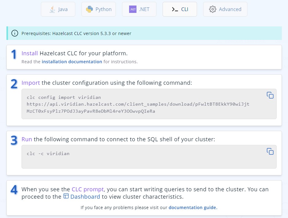
Select the CLI icon.

CLI icon

Follow the steps on the screen to download the CLC and the configuration for your cluster.

Step 4. Submit Job

Up to this point, you’ve used the SQL browser to run commands. This is useful for development and testing purposes, but in most production environments, you’ll create SQL scripts that you then submit to the cluster to run as jobs, using the CLC.

Clone the GitHub repo for this tutorial.
Change to the local directory for the repo.

Review the contents of the file connections_job.sql. You can use any text editor or the Linux more command.

more connections_job.sql

The JOIN part of this file is identical to the code you ran at the end of Step 2: Build and Test JOIN. The new code is at the beginning; instead of writing the search output to the screen, the output is stored in an IMap called live_connections.

To submit the script in non-interactive mode, use the following command.
```
clc -c <your-cloud-config> script run connections_job.sql
```
Don’t know the name of your cloud configuration? List available configurations using the following command.

clc config list
If you already have CLC open, you can submit the script from the CLC> prompt.
```
\script connections_job.sql
```

Watch the size of my-map increase as entries are written to it.

With a Standard or Dedicated license, you could view processing statistics and the DAG for this job as follows:

Go to the dashboard for your cluster and open Management Center.
In Management Center, select Stream Processing > Jobs.
Locate the job called update_connections.
Select the job name.

In either the SQL browser tab or the CLC, view the contents of the IMap that stores the output of the job.
```
SELECT * FROM live_connections;
```

Because you are searching the contents of an IMap, the results of the above SELECT are a "one and done" search. If you run the search multiple times, you will see different results, as the job is continuously updating the IMap. Your search will always display the latest data available at the time of the search.

Step 5. Run Client

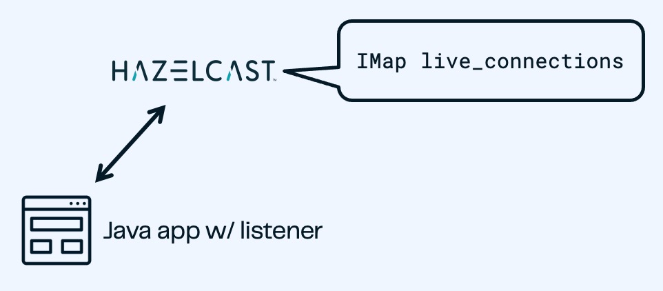
The connection data is now stored in Hazelcast and is being continually updated. Now let’s make that data available to the end application that will use it.

We’ve created a Java client that implements the Hazelcast map_listener function. The client connects to Hazelcast, retrieves the contents of the update_connections IMap, then updates the information any time there’s a change to the IMap.

Client diagram

Issue the following commands to build and launch the connection monitor application, replacing <cluster-name> with the name of the CLC cluster configuration.

cd connection-monitor
mvn clean package exec:java -Dexec.mainClass=hazelcast.platform.labs.airline.AirlineConnectionListener -Dexec.args=<cluster-name>

Hello Hazelcast testers! If you get an error regarding keystores with the above command, follow these steps:

Go to your Cloud cluster dashboard and select the Java client icon
Under "Advanced Setup", select "Download keystore file".
Find your CLC home directory with clc home.
Copy the zipped keystore to $CLC_HOME/configs/<your cluster name>
Unzip the keystore
Go back to the connection-monitor directory and try again.

Don’t worry - customers won’t have to do this; the next sprint will fix it so the keystore is downloaded with every config, not just Java.

Press CTRL+C to terminate the client connection.
(Optional) Open the Java file in your favorite IDE to review the client code.

Summary

In this tutorial/demo, you learned how to:

Connect to external data sources and sinks
Use SQL to search and display streaming data
Use SQL import data from an external database
Configure late event handling for streaming data
Join streaming and stored data to generate continually-updated results
Submit a job to Cloud using the Command Line Client